1 Mapper

The core of applying the projection space, cover, interval, and clustering is the Mapper algorithm. The Mapper algorithm takes in the original data, filter values, cover parameters, and clustering method to produce a simplicial complex that represents the structure of the original. The output includes an adjacency matrix representing the connections between nodes, the number of vertices (nodes), the level of each vertex, and the points contained in each vertex and level set.

knitr::include_graphics("./man/figures/mapper.png")

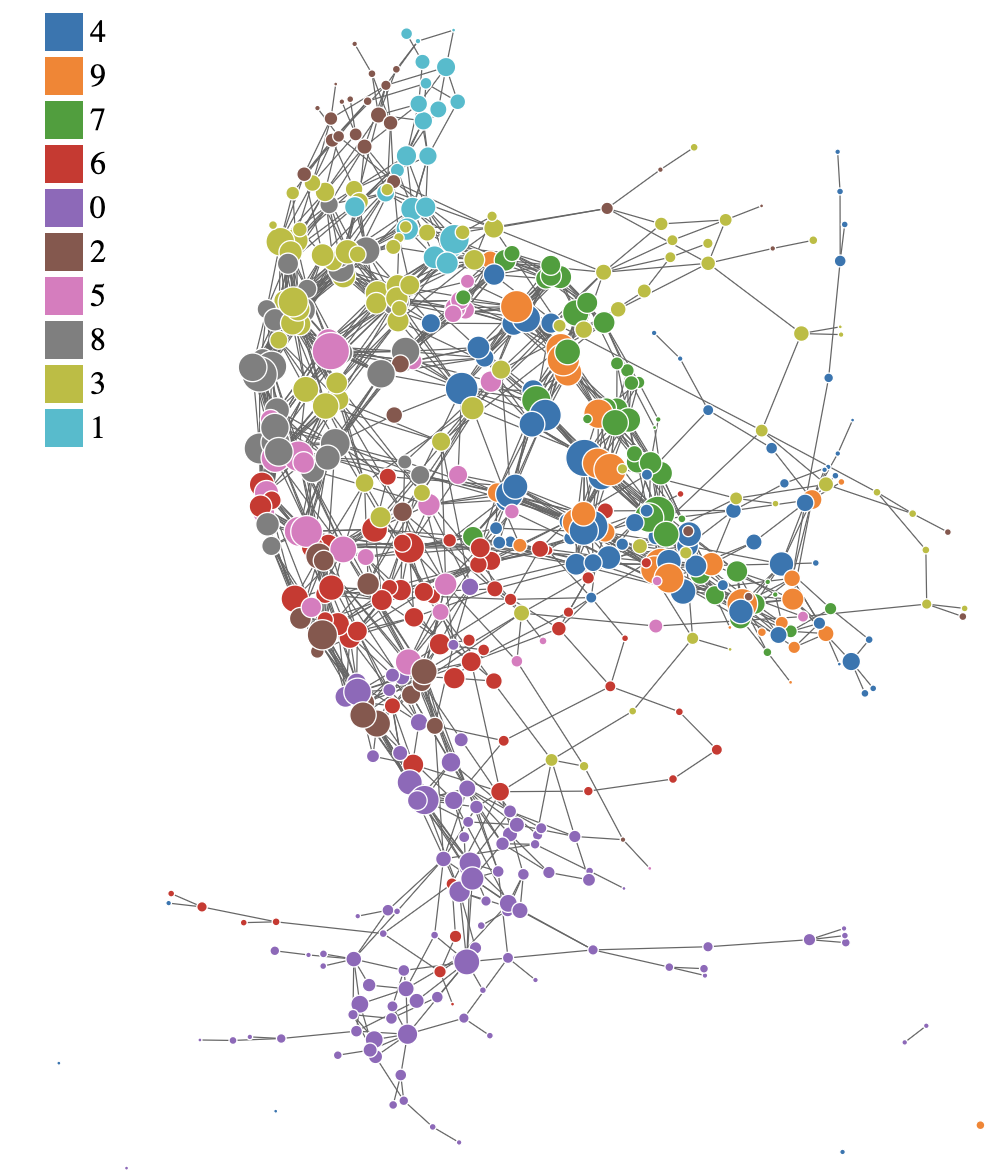
This is the example of the Mapper graph generated from the MNIST dataset. Each node represents a cluster of data points, and edges represent connections between clusters based on shared data points. The structure of the graph can reveal insights about the underlying data distribution and relationships between features.

knitr::include_graphics("./man/figures/MNISTMapper.png")

1.1 Example Code

library(ggplot2)
library(igraph)
library(networkD3)
library(parallel)
library(foreach)
library(doParallel)
library(htmlwidgets)
library(webshot)
library(tidygraph)
library(ggraph)

source('../../MapperAlgo/R/EdgeVertices.R')
source('../../MapperAlgo/R/ConvertLevelsets.R')
source('../../MapperAlgo/R/Cover.R')
source('../../MapperAlgo/R/Cluster.R')
source('../../MapperAlgo/R/SimplicialComplex.R')
source('../../MapperAlgo/R/MapperAlgo.R')

data("iris")
data <- iris

1.2 Run Mapper Algorithm

There are several clustering methods available, including DBSCAN, hierarchical clustering, k-means, and PAM. But you need to input all of the params required for the chosen method in method_params.

time_taken <- system.time({
  Mapper <- MapperAlgo(
    original_data = data[,1:4],
    filter_values = data[,1:2],
    # filter_values = circle_data[,2:3],
    percent_overlap = 30,
    methods = "dbscan",
    method_params = list(eps = 1, minPts = 1),
    # methods = "hierarchical",
    # method_params = list(num_bins_when_clustering = 10, method = 'ward.D2'),
    # methods = "kmeans",
    # method_params = list(max_kmeans_clusters = 2),
    # methods = "pam",
    # method_params = list(num_clusters = 2),
    cover_type = 'stride',
    # intervals = 4,
    interval_width = 1,
    num_cores = 12
    )
})
time_taken

1.2.1 MapperAlgo Params

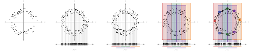
MapperAlgo funtion remains several params, filter_values is the data you get after pojection, for example, the output of PCA. Intervals is how many areas you want, in the example below, you cut the data into 4 areas, and the 4 areas will be ovelapped in 30%, then it will calculate the width for you. You can also choose interval_width as input, but you can’t use it and Intervals at the same time because it will cause nonuniform intervals in space, vice versa.

You can choose hierarchical, kmeans, dbscan, or pam in methods, and according to their original package, you must input a list of params to method_params. Then, according to the original author and the paper, stride or extension in cover_type can be choose in the function, more informations are explained in File explaination. The num_cores can be set depend on how many cores you want to use for parrallel computing.

MapperPlotter is just plotting the nodes and edges, use forceNetwork if you want to interact with the plot, and ggraph could get you more informations in label. avg will give you the mean feature of each node if you set it as TRUE, in the example below, circle_data$circle is the feature.

1.2.2 Output data

Name	Context
adjacency	24x24 adjacency matrix, 0 or 1
num_vertices	Mapper nodes num
level_of_vertex	Each node represent to which level set index, correspond to intervals.
points_in_vertex	Each node carries original data index
points_in_level_set	Each level set(16) include data point index, level set represent data subset in a lens function
vertices_in_level_set	Which node represent to a level set

1.3 Plots

There are built-in plotting functions to visualize the Mapper graph. You can choose between “ggraph” and “forceNetwork” types. Additionally, you can choose to average feature values over nodes or use conditional probability embeddings.

source('../../MapperAlgo/R/Plotter.R')

g <- graph_from_adjacency_matrix(Mapper$adjacency, mode = "undirected")
e_result <- eigen_centrality(g)
MapperPlotter(Mapper, label=e_result$vector, original_data=data, avg=FALSE, use_embedding=TRUE)

1.4 Correlation between Mapper graph and features

Sometimes it is useful to find out whether the Mapper graph structure correlates with certain features in the data. For example, if Sepal.Length densities are similar to Sepal.Width densities across the nodes in the Mapper graph.

source('../../MapperAlgo/R/MapperCorrelation.R')
MapperCorrelation(Mapper, original_data = original_data, labels = list(data$Sepal.Length, data$Sepal.Width))

1.5 Grid Search for optimal cover parameters

If you want to find optimal cover parameters for your data, you can use the GridSearch function. Observing the convergence of certain graph metrics as cover parameters change can help you select appropriate values.

source('../../MapperAlgo/R/GridSearch.R')
cpe_params <- list("PW_group", "Species", "wide", "versicolor")
data$PW_group <- ifelse(data$Sepal.Width > 1.5, "wide", "narrow")
labels <- data%>%select(PW_group, Species)
GridSearch(
  filter_values = data[,1:4],
  label = labels,
  column = "Species",
  cover_type = "stride",
  width_vec = c(1),
  overlap_vec = c(30),
  num_cores = 12,
  out_dir = "../mapper_grid_outputs",
  avg = TRUE,
  use_embedding = cpe_params
)